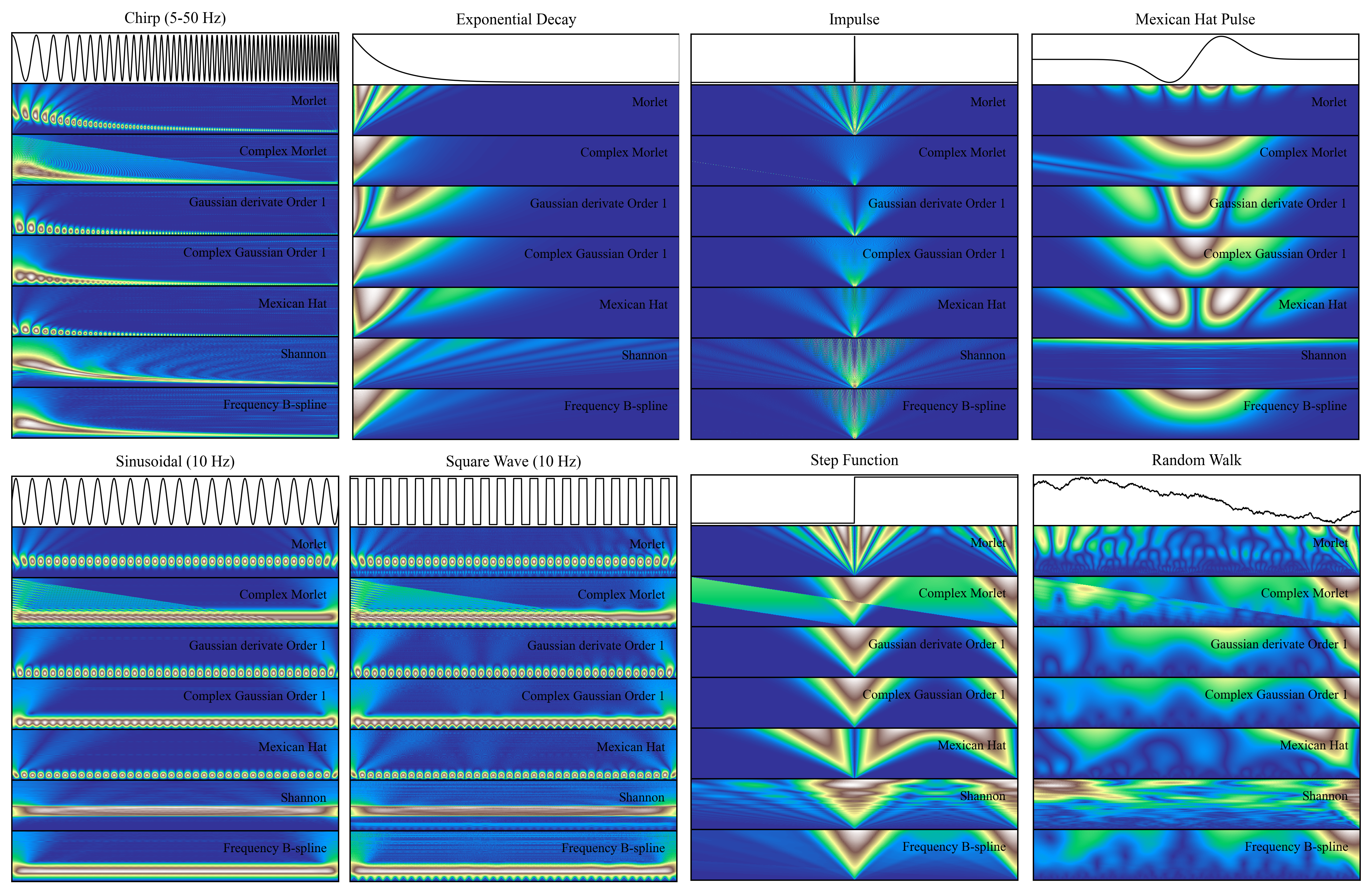
Which wavelet is best for my signal? The answer depends on the nature of your data and what features you’re trying to extract. Wavelets are mathematical functions that decompose signals into time-frequency space. Each wavelet has its own shape, symmetry, and localization properties. Choosing the best wavelet means finding one whose characteristics align with the structure of your signal. For example, if you’re analyzing a sinusoidal signal, the Morlet wavelet which resembles a localized sine wave is a natural fit. It offers excellent frequency resolution and produces a scalogram with clean, horizontal bands. If you’re working with transient features like spikes or impulses, wavelets like the Mexican Hat or Gaussian derivatives are better suited. These wavelets are sharply localized in time and highlight sudden changes with precision.
The visual output of a wavelet transform should reveal the signal’s key features clearly on a scalogram. For periodic signals, you want consistent frequency bands. For chirps, you expect diagonal ridges that track frequency changes over time. For impulses, you look for sharp vertical bursts across scales.
Ultimately, the appropiate wavelet is one that makes your signal’s structure most interpretable. It minimizes artifacts, enhances relevant features, and aligns with the goals of your analysis—whether that’s classification, denoising, or feature extraction. Wavelet selection isn’t just a technical choice—it’s a creative one. It’s about matching the lens to the landscape. And once you find the right fit, your signal’s hidden story becomes beautifully clear.
Discrete Wavelet Transform
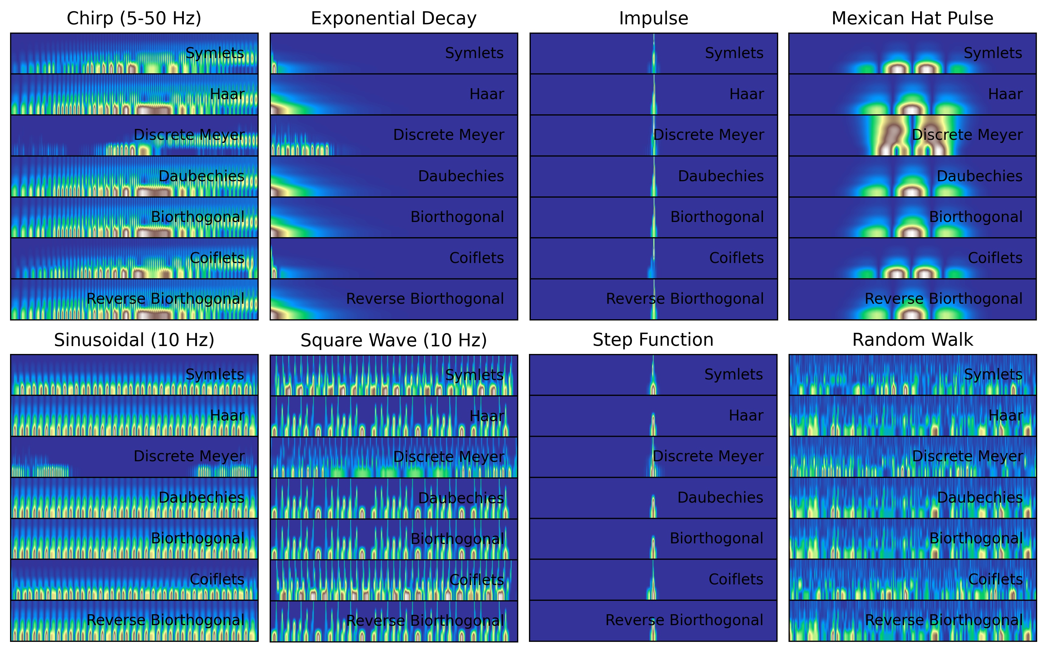
Scalograms offer fine-grained resolution and are ideal for visualizing how frequency content evolves continuously over time. In contrast, Discrete Wavelet Transform operates on dyadic scales—powers of two, and uses filter banks to decompose the signal into hierarchical levels. Each level captures either coarse approximations or fine details, and the signal is downsampled at each stage. When visualized as a heatmap, DWT coefficients show energy across discrete levels, but lack the continuous time-frequency resolution of a scalogram.
The result is a blocky, level-based heatmap that reflects the structure of the decomposition rather than a smooth frequency sweep. These heatmaps are excellent for tasks like compression, denoising, and feature extraction, but they don’t represent frequency evolution in the same way scalograms do. In short, scalograms provide a continuous view of signal dynamics, while DWT heatmaps offer a compact, multi-resolution snapshot.
Customize Wavelets
Choosing the right wavelet family is only half the equation — tuning its parameters is just as critical. Many continuous wavelets, like Morlet, Complex Morlet, Shannon, and Frequency B-Spline, are not fixed shapes but flexible templates. Parameters such as central frequency (w), bandwidth (fb), and center frequency (fc) define how the wavelet behaves in time and frequency domains.
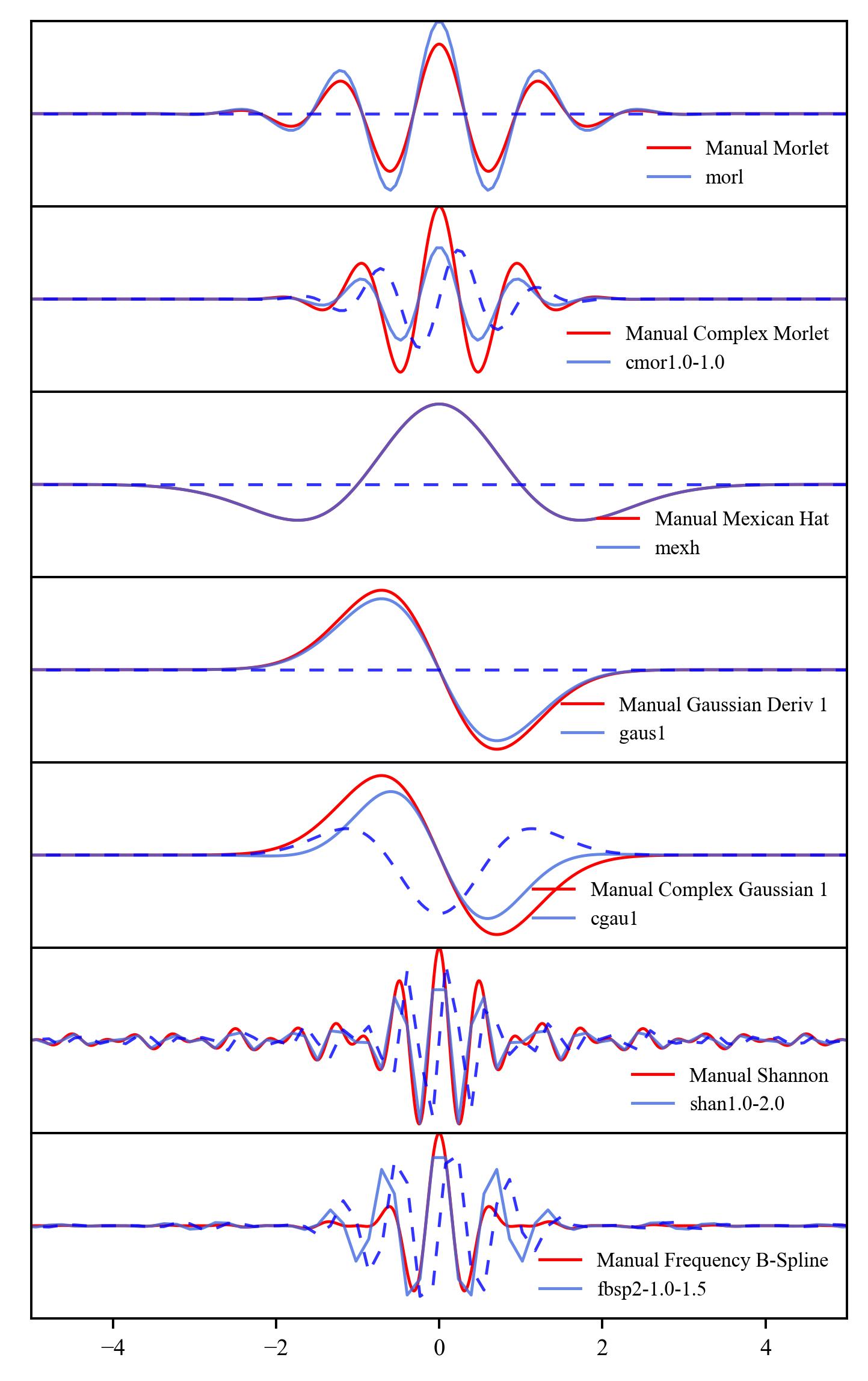
Using default parameters blindly can lead to missed features in your signal, misinterpretation of the scale-frequency relationship, and poor resolution in either time or frequency. These defaults may not align with the specific characteristics of your data. However, when you tune the wavelet parameters intentionally, you gain the ability to zoom in on fast transients, stretch out slow rhythms, and match the wavelet to your signal’s dominant patterns — dramatically improving the clarity and relevance of your analysis.